# Importing genotypic data
geno_file <- 'data/barley_genbank_2388variants_554individuals_biallelic.hmp.txt.gz'

geno_data <- read.csv(geno_file, sep = "\t")

# Show the first 50 rows/columns only
create_dt(geno_data[1:50,1:50])20 Module 6.1: Genomic Selection
Genomic selection enables early and accurate prediction of complex traits based on genome-wide SNP data. This can allow us to predict performance immediately after genotyping seedlings, which can speed up selection decisions and reduce the cost of field trials. We will be using the rrBBLUP package for this part, which is a is a package for genomic prediction with the ridge regression best linear unbiased prediction or RR-BLUP mixed linear model (Endelman, 2011). One application is to estimate marker effects by ridge regression; alternatively, BLUPs can be calculated based on an additive relationship matrix or a Gaussian kernel.
20.1 Read, Filter and Impute Marker Data
The genotypic matrix for rrBLUP has to be coded as {-1, 0, 1}, meaning we will need a conversion step if our data is not yet in that format. Moreover, we will be carrying out a mean value imputation.
M <- geno_data[, -c(1:11)]
rownames(M) <- geno_data[, 1]
M <- t(M)

# Reformatting matrix to numeric
M <- ASRgenomics::snp.recode(M, na.string = 'NN', rename.markers = FALSE)$Mrecode
A total of 87800 values were identified as missing with the string NN and were replaced by NA.Matrix M was recoded from bi-allelic nucleotide bases to numeric.# Filtering genotypic matrix
M <- ASRgenomics::qc.filtering(M,
marker.callrate = 0.1,
ind.callrate = 0.2,
maf = 0.05,
impute = TRUE)$M.cleanInitial marker matrix M contains 554 individuals and 2388 markers.A total of 674 markers were removed because their proportion of missing values was equal or larger than 0.1.A total of 5 individuals were removed because their proportion of missing values was equal or larger than 0.2.A total of 34 markers were removed because their MAF was smaller than 0.05.A total of 0 markers were removed because their heterozygosity was larger than 1.A total of 0 markers were removed because their |F| was larger than 1.Final cleaned marker matrix M contains 2.84% of missing SNPs.Final cleaned marker matrix M contains 549 individuals and 1680 markers.A total of 26221 missing values were imputed, corresponding to 2.84% of the total number of SNPs.# Reformatting to required format
M <- as.matrix(M) - 1
# Show the first 50 rows/columns only
create_dt(M[1:50,1:50])20.2 Read and Align Phenotypic Data
# Importing phenotypic data
pheno_file <- 'barley_genbank_phenotypic_mean_data.csv'

pheno_data <- read.csv(pheno_file)

pheno_data <- merge(pheno_data, as.data.frame(rownames(M)), by.x = 'sample_id', by.y = 1, all.y = TRUE)

# Extracting requires trait
y <- pheno_data$Yield

# Printing phenotypic data
create_dt(pheno_data)
20.3 Model 1
The first model assumes that all marker effects are normally distributed and have identical variance. Parameters are estimated as a solution to the optimization problem. Predictions from this method are equivalent to BLUP values from an animal model (i.e., GBLUP). The observed relationship matrix is calculated from the markers using the formula by VanRaden (2008).
# Fitting a Model using rrBLUP (case 1: all SNPs in the random effect)
GS <- rrBLUP::mixed.solve(y, Z = M, X = NULL, method = 'REML')

# Obtaining predictions
predGS <- matrix(data = GS$beta, nrow = length(y), ncol = 1) + M %*% GS$u

# Printing predictions
create_dt(cbind(round(predGS, 3), y))
# Plotting predictions
plot(y, predGS)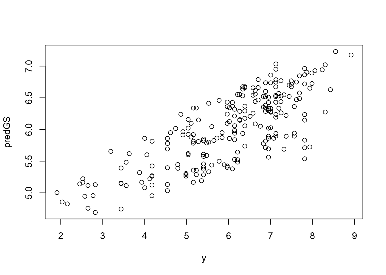
20.3.1 Goodness of Fit Statistics
# Heritability
# Trait variance
(var_y  <- var(y, na.rm = TRUE))
[1] 2.107743# Error variance
(var_e <- GS$Ve)[1] 1.465679# Proportion of explained variance (High = good fit, potential heritability)
(h2_GS <- 1 - var_e / var_y)[1] 0.3046215Anas_table <- cbind(rownames(M), y, predGS)
# Predictive ability (High = good prediction accuracy)
(PA <- cor(y, predGS, method = 'pearson', use = 'complete.obs')) [,1]
[1,] 0.780012520.4 Model 2
This model handles some markers as having a fixed effect (e.g. significant SNPs from GWAS output). It splits the genotypic data into X matrix (fixed effects) and Z matrix (random effects). To calculate the REML solution for the model you solve y = X b + Z u + e. We predict BLUE(b) and BLUP(u) solutions for the fixed and random effects, respectively, using standard formulas (Searle et al. 1992).
# Defining markers
markers <- c('S7H_63131260', 'S5H_573915992')
SNPs    <- colnames(M)

# Filtering matrices
X <- M[, SNPs %in% markers]
Z <- M[,!SNPs %in% markers]

# Fitting a Model using rrBLUP by exclude markers from the Z matrix (for the Random effects) and include them in the X matrix (for the fixed effect)
GS <- rrBLUP::mixed.solve(y, Z = Z, X = X, method = 'REML')

# Obtaining predictions
predGS <- X %*% GS$beta + Z %*% GS$u

# Printing predictions
create_dt(cbind(round(predGS, 3), y))
# Plot to verify
plot(y, predGS)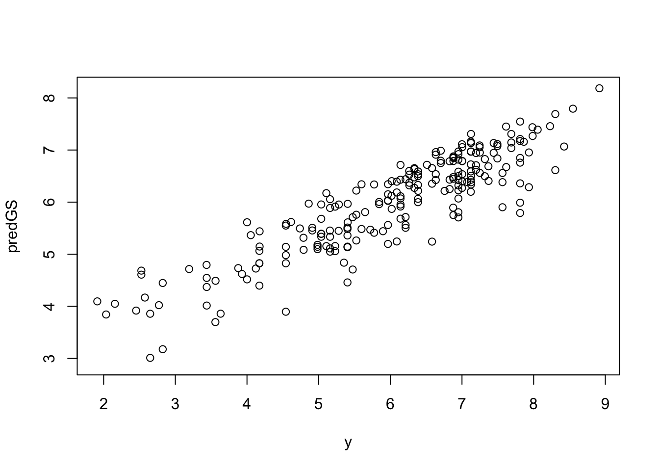
20.4.1 Goodness of Fit Statistics
# Heritability (GS)
# Trait variance
(var_y <- var(y, na.rm = TRUE))[1] 2.107743# Error variance
(var_e <- GS$Ve)[1] 1.018018# Proportion of explained variance (High = good fit, potential heritability)
(h2_GS <- 1 - var_e / var_y)[1] 0.5170105# Predictive Ability (correlation between actual and predicted response)
(PA <- cor(y, predGS, method = 'pearson', use = 'complete.obs')) [,1]
[1,] 0.895261420.5 K-Fold Cross Validation
# Set the total number of folds, and get the total number of individuals
k <- 5
n <- length(y)
# Set randomly the fold group for each observation
# That tells when it will be used for validation
group <- sample(rep(1:k, length.out = n), n)
head(group, 20) [1] 5 1 3 2 1 4 2 4 1 4 4 4 2 4 3 3 2 5 1 5table(group)group
1 2 3 4 5
110 110 110 110 109 # An empty matrix to save calculated heritability in each fold, and GS prediction that calculated when individual be in validation group
predGS <- matrix(data = NA, nrow = n, ncol = 1)
h2_cv <- matrix(data = NA, nrow = k, ncol = 1)
for (g in 1:k) {
# Reset response variable, and exclude validation set values for the given k fold
y_cv <- y
y_cv[group == g] <- NA
# Fitting a Model using rrBLUP (model 1: all SNPs in the random effect)
# GS <- mixed.solve(y_cv, Z = M, X = NULL, method = 'REML')
# predGS_cv <- matrix(data = GS$beta, nrow = length(y), ncol = 1) + M %*% GS$u
# Model 2: have some markers to be handled as a fixed effect
GS <- rrBLUP::mixed.solve(y_cv, Z = Z, X = X, method = 'REML')
# Obtaining predictions
predGS_cv <- X %*% GS$beta + Z %*% GS$u
# Heritability (GS)
var_y <- var(y_cv, na.rm = TRUE)
var_e <- GS$Ve
h2_cv[g] <- 1 - var_e / var_y
# Get the GS prediction for all validation set individuals
predGS[group == g] <- predGS_cv[group == g]
}
# Plot to verify
plot(y, predGS)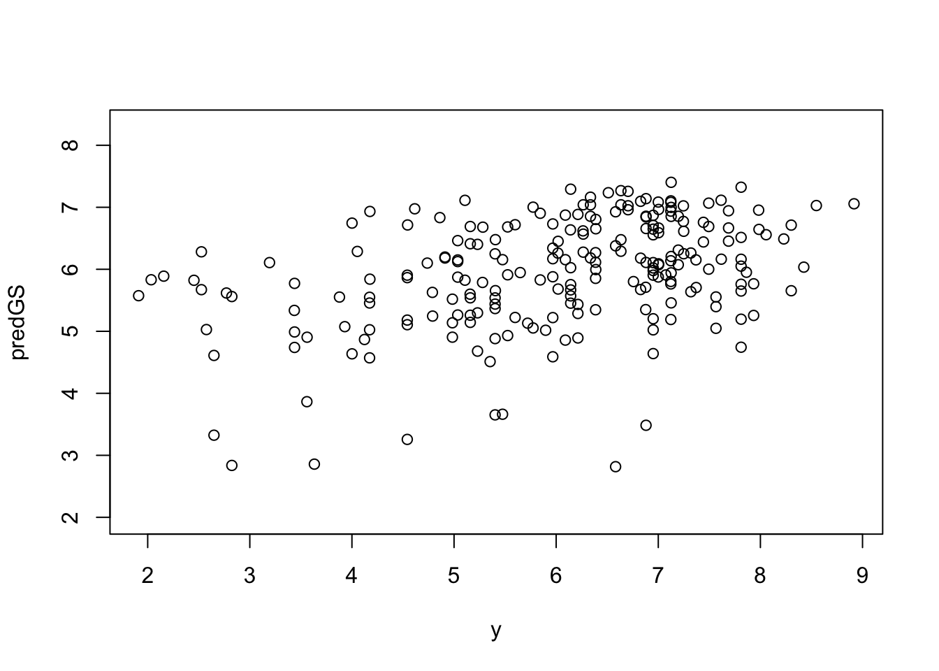
# Heritability (GS cross-validation)
h2_cv
[,1]
[1,] 0.5669156
[2,] 0.4867977
[3,] 0.5506054
[4,] 0.5487734
[5,] 0.5748752mean(h2_cv)[1] 0.5455935# Predictive Ability (correlation between actual and predicted response)
(PA <- cor(y, predGS, method = 'pearson', use = 'complete.obs')) [,1]
[1,] 0.39847920.6 Predict Breeding Values
# Calculate the additive relationship matrix (it is the kinship matrix multiplied by 2) it can also perform imputation for missing marker data by
# Define impute.method (mean or EM) (see also: min.MAF, max.missing, and return.imputed parameters)
A <- rrBLUP::A.mat(M)
heatmap(A)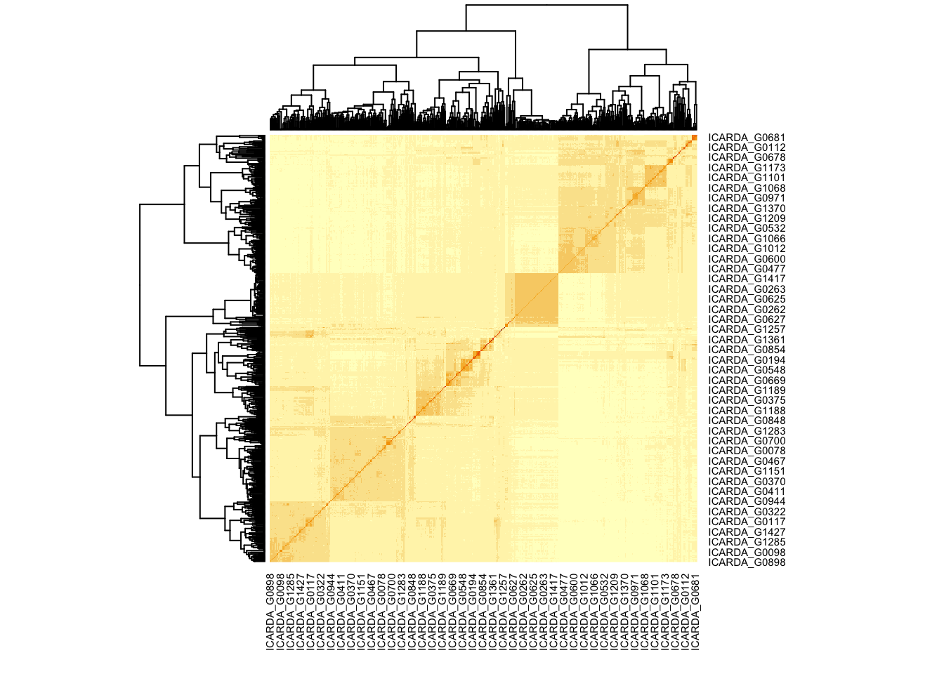
GS <- rrBLUP::mixed.solve(y, K = A.mat(M), SE = TRUE)

# Genomic Estimated Breeding Value (GEBV)
GEBV <- cbind(round(GS$u, 3), round(GS$u.SE, 3))

colnames(GEBV) <- c('GEBV', 'SE')

create_dt(GEBV)