# File paths for data import
geno_file  <- 'data/Raw_SNPS_80_Present_5_MAF.hmp.txt'
pheno_file <- 'data/Pheno_REML.csv'
trait_name <- 'ASC_Score'18 Module 5.1: Introduction to GWAS
The purpose of Genome-Wide Association Studies (GWAS) is to identify genetic variants associated with specific traits. We will be using the statgenGWAS package, which has been designed for performing single trait GWAS.
18.1 Reading the Marker Matrix
Markers can either be coded as character strings or as numerical values. Common coding styles include the following options:
AA, AB, BA, BB -> 0, 1, 1, 2 (A is reference allele, and B is alternative allele)
CC, CT, TC, TT -> 0, 1, 1, 2 (e.g., ref. allele is C)
C, Y, Y, T -> 0, 1, 1, 2 (Nucleic Acid Notation)
numerical code: 0, 1, 1, 2 (0 ref./major allele, 2 alt./minor allele, and 1 is heterozygous) statgenGWAS
numerical code: -1, 0, 0, 1 (-1 ref./major allele, 1 alt./minor allele, and 0 is heterozygous) rrBLUP
genotypic_data <- read.table(geno_file,
                             header = TRUE,
                             comment.char = '')

# Show the first 50 rows/columns only
create_dt(genotypic_data[1:50,1:50])
18.1.1 Marker Map
The data.frame map is used to describe the physical positions of the markers on the chromosomes. The data consists of two columns, chr for the name or number of the chromosome and pos for the position of the marker on the chromosome. The position can be in basepair or in centimorgan. The names of the markers should be the row names of the data.frame.
marker_map <- genotypic_data[, 3:4]
colnames(marker_map) <- c('chr', 'pos')
rownames(marker_map) <- genotypic_data[, 1]

create_dt(marker_map)
18.1.2 Marker Matrix
The marker matrix is stored in the matrix marker within the gData object. It has the names of the markers in its column names and the genotypes in its row names. Markers can either be coded as character strings or as numerical values. Important note, before performing any analysis, the marker matrix has to be converted to a numerical matrix. This can be do using the function codeMarkers.
marker_matrix <- genotypic_data[, -c(1:11)]
rownames(marker_matrix) <- genotypic_data[, 1]
marker_matrix <- t(marker_matrix)

# show the first 50 rows/columns only
create_dt(marker_matrix[1:50,1:50])
We can use the marker map and marker matrix to create a gData object.
gData <- createGData(geno = marker_matrix, map = marker_map)18.1.3 Recording and Cleaning of Data
Marker data has to be numerical and without missing values in order to do GWAS analysis. This can be achieved using the codeMarkers() function. In this example our marker matrix is not numerical; however, the function also allows us to input an already numerical matrix for filtering and the imputation of missing values.
codeMarkers(gData, naStrings = NA, impute = TRUE, verbose = TRUE, nMiss = 1, nMissGeno = 1, MAF = NULL, imputeType): returens a copy of the input gData object with markers replaced by coded and imputed markers
naStings: character vector of strings to be treated as NAimpute: defaults to TRUE, performs imputation of missing valuesverbose: defaults to TRUE, prints a summary of performed stepsnMiss: a numerical value between 0 and 1, SNPs with a fraction of missing values higher than this value will be removednMissgeno: a numerical value between 0 and 1, genotypes with a fraction missing values higher than this value will be removedMAF: a numerical value between 0 and 1, SNPs with a MAF below this value will be removedimputeType: indicates type of imputation ("fixed","random","beagle")
# Remove duplicate SNPs from gData
gData <- codeMarkers(gData,
                     naStrings = 'N',
                     removeDuplicates = TRUE,
                     impute = FALSE,
                     verbose = TRUE)
Input contains 2772 SNPs for 200 genotypes.
43190 values replaced by NA.
0 genotypes removed because proportion of missing values larger than or equal to 1.
0 SNPs removed because proportion of missing values larger than or equal to 1.
467 duplicate SNPs removed.
Output contains 2305 SNPs for 200 genotypes.# SNPs with a fraction of missing values higher than nMiss will be removed.
gData <- codeMarkers(gData,
impute = FALSE,
verbose = TRUE,
nMiss = 0.1)Input contains 2305 SNPs for 200 genotypes.
0 genotypes removed because proportion of missing values larger than or equal to 1.
634 SNPs removed because proportion of missing values larger than or equal to 0.1.
0 duplicate SNPs removed.
Output contains 1671 SNPs for 200 genotypes.# Genotypes with a fraction of missing values higher than nMissGeno will be removed.
gData <- codeMarkers(gData,
impute = FALSE,
verbose = TRUE,
nMissGeno = 0.2)Input contains 1671 SNPs for 200 genotypes.
12 genotypes removed because proportion of missing values larger than or equal to 0.2.
0 SNPs removed because proportion of missing values larger than or equal to 1.
318 duplicate SNPs removed.
Output contains 1353 SNPs for 188 genotypes.# SNPs with a Minor Allele Frequency (MAF) below this value will be removed.
gData <- codeMarkers(gData,
impute = FALSE,
verbose = TRUE,
MAF = 0.05)Input contains 1353 SNPs for 188 genotypes.
0 genotypes removed because proportion of missing values larger than or equal to 1.
0 SNPs removed because proportion of missing values larger than or equal to 1.
36 SNPs removed because MAF smaller than 0.05.
0 duplicate SNPs removed.
Output contains 1317 SNPs for 188 genotypes.To decide how we wish to impute our data we can evaluate the total number of remaining missing values and their ratio. We can choose between the following imputation types:
fixed: Impute all missing values by a single fixed value. Use the parameter fixedValue to set this value
random: Impute missing values with a random value based on the non-missing values for a SNP, OK when ratio of missing values is less than 5%.
beagle: Impute missing values using the independent beagle software (Browning and Browning 2007)
(d <- dim(gData$markers))[1] 188 1317(n <- sum(is.na(gData$markers)))[1] 3036(r <- n/(d[1]*d[2]))[1] 0.01226191In this case we will carry out our missing value imputation using the beagle method.
set.seed(42)
gData <- codeMarkers(gData,
                     impute = TRUE,
                     imputeType = 'beagle',
                     verbose = TRUE)
Input contains 1317 SNPs for 188 genotypes.
0 genotypes removed because proportion of missing values larger than or equal to 1.
0 SNPs removed because proportion of missing values larger than or equal to 1.
0 duplicate SNPs removed.
3036 missing values imputed.
230 duplicate SNPs removed after imputation.
Output contains 1087 SNPs for 188 genotypes.18.1.4 Plot Genetic Map
plot(gData)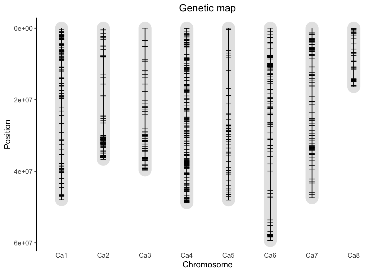
18.2 Reading the Phenotypic Data
Phenotypic data, either directly from field trials or after summarizing can be stored in pheno in the gData object. Pheno can either be a single data.frame or a list of data.frames for storing data for different trials or different summarizations of the original data. The first column of all elements of pheno should be genotype and all the other columns should represent different traits. Storing additional variables should be done in covar.
# Import phenotypic data
phenotypic_data <- read.csv(pheno_file)
colnames(phenotypic_data) <- c('genotype', trait_name)

# Add phenotypic data to gData
gData <- createGData(gData, pheno = phenotypic_data)
18.3 Summarize gData
summary(gData)map
Number of markers: 1087
Number of chromosomes: 8
markers
Number of markers: 1087
Number of genotypes: 188
Content:
0 1 2 <NA>
0.75 0.25 0.00 0.00
pheno
Number of trials: 1
phenotypic_data:
Number of traits: 2
Number of genotypes: 200
ASC_Score NA
Min. 0.9400 1.156000
1st Qu. 3.9600 1.189750
Median 4.9300 1.209000
Mean 4.9652 1.207365
3rd Qu. 6.1250 1.223000
Max. 8.8200 1.288000
NA's 0.0000 0.000000