We will be carrying out the GWAS analysis using the runSingleTraitGwas() function from the statgenGWAS package.
runSingleTraitGwas(gData, traits = NULL, covar = NULL, snpCov = NULL, kin = NULL, kinshipMethod, remlAlgo, GLSMethod, MAF = 0.01, thrType, alpha = 0.05, LODThr = 4, nSnpLOD = 10, pThr = 0.05): performs a single-trait Genome Wide Association Study (GWAS) on phenotypic and genotypic data contained in a gData object.
gData: an object of class gData
traits: vector of traits on which to run GWAS (numeric indices or character names)
covar: defaults to NULL, an optional vector of covariates taken into account when running GWAS. These can be either numeric indices or character names of columns in covar in gData
snpCov: an optional character vector of snps to be included as covariates
kin: an optional kinship matrix or list of kinship matrices
kinshipMethod: optional character indicating the method used for calculating the kinship matrix(ces). Currently "astle" (Astle and Balding, 2009), "IBS" and "vanRaden" (VanRaden, 2008) are supported
remlAlgo: character string indicating the algorithm used to estimate the variance components. Either EMMA, for the EMMA algorithm, or NR, for the Newton-Raphson algorithm
GLSMethod: character string indicating the method used to estimate the marker effects
MAF: numerical value between 0 and 1. SNPs with MAF below this value are not taken into account
thrType: character string indicating the type of threshold used for the selection of candidate loci
alpha: defaults to 0.05, numerical value used for calculating the LOD-threshold for thrType = “bonf” and the significant p-Values for thrType = “fdr”
LODThr: numerical value used as a LOD-threshold when thrType = "fixed"
nSnpLOD: numerical value indicating the number of SNPs with the smallest p-values that are selected when thrType = “small”
pThr: numerical value just as the cut off value for p-Values for thrType = "fdr"
19.1 Significance Threshold
Prior to running our analysis, we need to compute a threshold by which to identify significant SNPs. The threshold for selecting significant SNPs in a GWAS analysis tends to be computed by using Bonferroni correction, with an alpha of 0.05. The alpha can be modified by setting the option alpha when calling the runSingleTraitGwas() function. Two other threshold types can be used: a fixed threshold (we set the thrType parameter to “fixed”) by specifying the log10(p) (LODThr) value of the threshold, or a small threshold (we set the thrType parameter to “small” and nSnpLOD to n) which defines the n SNPs with the highest log10(p) scores as significant SNPs.
There are two ways to compute the phenotypic variance covariance matrix used in the GWAS analysis. Either the EMMA algorithm (Kang et al. 2008) or the Newton-Raphson algorithm (Tunnicliffe 1989). Specify the method by setting the parameter remlAlgo to either “EMMA” or “NR”. By default the EMMA algorithm is used.
Note that the estimated effect is computed for a single allele. Its direction depends on the coding of the markers in the gData object. In this example the minor allele was used as reference allele, so the effects are the estimated effects for the minor allele.
19.4 Significant Alleles
signSnp is a data.tables containing the significant SNPs. Optionally, the SNPs close to the significant SNPs are included in the data.table. The data.table in signSnp consist of the same columns as those in GWAResult described above. Two extra columns are added:
snpStatus: either significant SNP or within … of a significant SNP
propSnpVar: proportion of the variance explained by the SNP
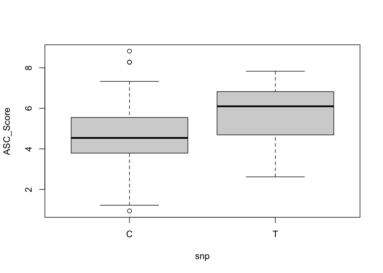
We can manually check by using t.test, which is the old school way.
# Creating data frame for t-testdf <-as.data.frame(marker_matrix[,snp])df$genotype <-rownames(marker_matrix)colnames(df) <-c('snp', 'genotype')df <-merge(df, phenotypic_data, id ='genotype')df <-na.omit(df)table(df$snp)
    Welch Two Sample t-test

data:  ASC_Score by snp
t = -5.4233, df = 114.29, p-value = 3.308e-07
alternative hypothesis: true difference in means between group C and group T is not equal to 0
95 percent confidence interval:
 -1.6581884 -0.7709251
sample estimates:
mean in group C mean in group T
       4.592171        5.806727
# Plotting t-test resultsboxplot(formula(paste(trait_name, '~ snp')), data = df)
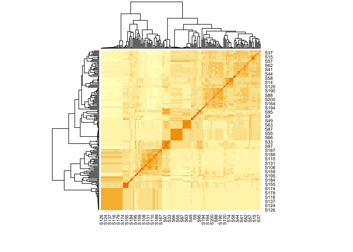
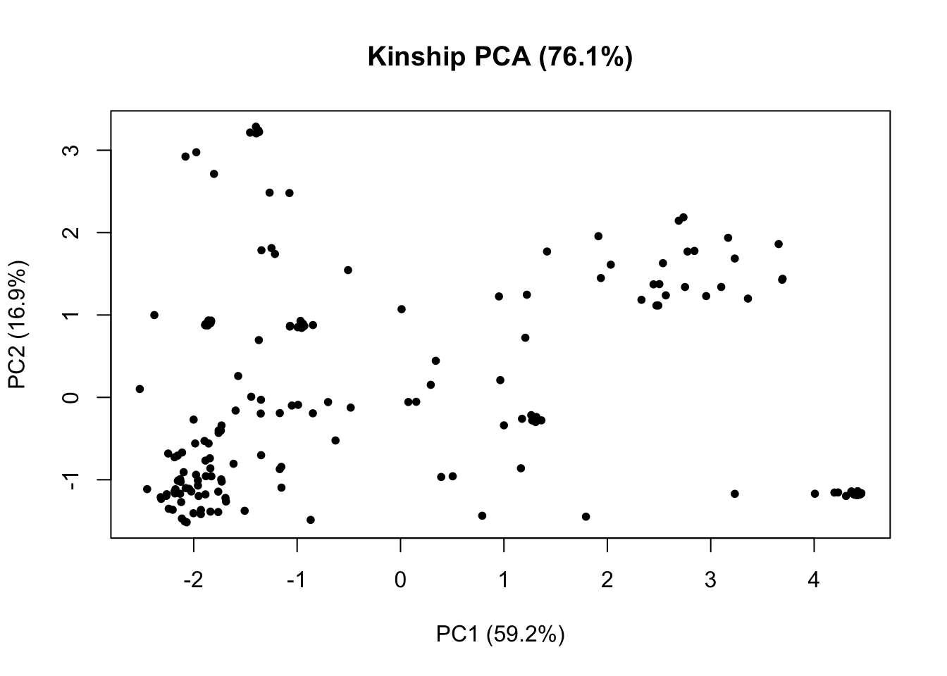
19.5 Kinship Results
A kinship matrix was produced and used in the GWAS analysis. The method for producing this matrix can be defined by thge kinshipMethod parameter in the runSingleTraitGwas() function. By default, the same kinship matrix is used for testing all SNPs (GLSMethod = “single”). When GLSMethod = “multi”, the kinship matrix is chromosome-specific. As shown by Rincent et al.(2014), this often gives a considerable improvement in power.
General information of our GWAS results can be obtained by printing the GWASInfo part of our GWAS object. GWASInfo$inflationFactor returns the inflation factor (Devlin and Roeder 1999). Ideally this factor should be 1, meaning there is no inflation at all. If the values are further away from 1, the inflation can be corrected for by setting genomicControl = TRUE in runSingleTraitGwas().
For a quick overview of the results, e.g. the number of significant SNPs, use the summary function.
summary(GWAS)
phenotypic_data:
    Traits analysed: ASC_Score

    Data are available for 1087 SNPs.
     0 of them were not analyzed because their minor allele frequency is below 0.01

    GLSMethod: single
    kinshipMethod: vanRaden

    Trait: ASC_Score

        Mixed model with only polygenic effects, and no marker effects:
        Genetic variance: 0.646051
        Residual variance: 1.895564

        LOD-threshold: 3.5
        Number of significant SNPs: 2
        Smallest p-value among the significant SNPs: 6.81679e-05
        Largest p-value among the significant SNPs: 0.0002511666 (LOD-score: 3.600038)

        No genomic control correction was applied
        Genomic control inflation-factor: 0.885
19.8 Plots
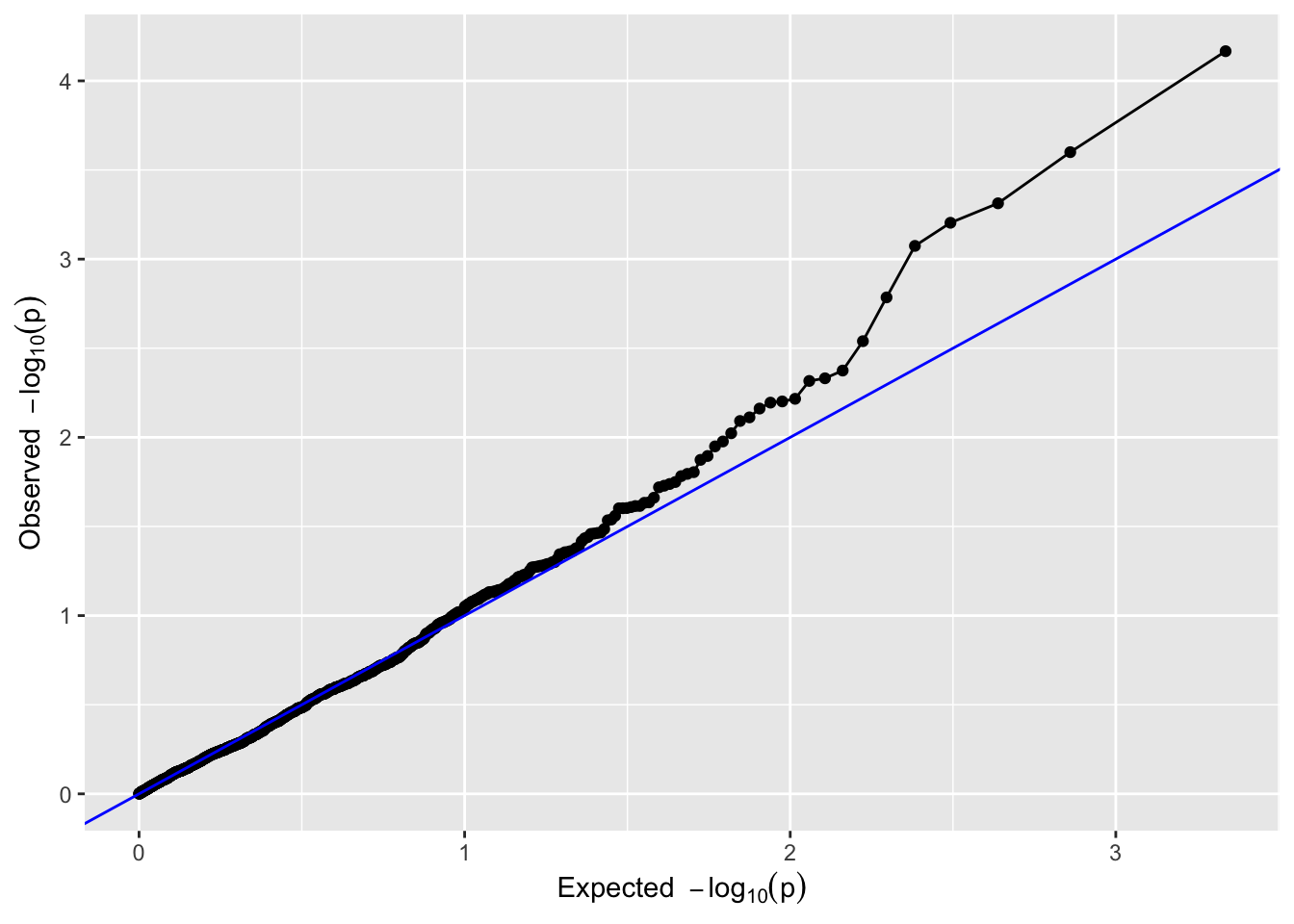
19.8.1 QQ-Plot
A QQ-plot of the observed against the expected log10(p) values. Most of the SNPs are expected to have no effect, resulting in P-values uniformly distributed on [0,1], and leading to the identity function (y=x) on the log10(p) scale. Deviations from this line should only occur on the right side of the plot, for a small number of SNPs with an effect on the phenotype (and possibly SNPs in LD).
plot(GWAS, plotType ='qq', trait = trait_name)
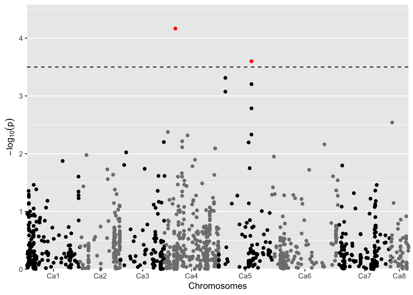
19.8.2 Manhattan Plot
A Manhattan plot of GWAS. Significant SNPs are marked in red. Plot only 5% of SNPs with a LOD below 2 (lod = 2)
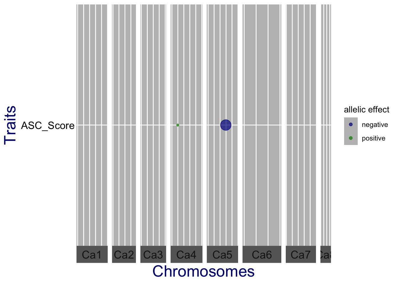
A qtl plot of GWAS. The significant SNPs are marked by circles at their genomic positions, with diameter proportional to the estimated effect size. Colors indicate the direction of the effect: green when the allele increases the trait value, and blue when it decreases the value.