# Importing our genotypic data
raw_matrix <- read.table("data/BarleyMatrix.txt", sep = "\t", header = TRUE, row.names = 1, check.names = FALSE)14 Module 4.1: Kinship and Relatedness
Identifying relatedness between individuals is important to ensure samples are independent, as not accounting for kinship may distort posterior analyses such as GWAS or population structure. Kinship coefficients can help control confounding affects in association studies and can help infer subpopulations when studying structure. Moreover, not only may individuals be related, we can sometimes find duplicates of the same individual, which can skew posterior diversity estimates. Overall, studying kinship allows us to maintain the quality standard of our data.
14.1 Kinship
Kinship refers to the genetic relatedness between individuals, and it is a measure of how much of their genomes two individuals share due to common ancestry. Kinship is often evaluated by calculating a kinship matrix. We can use the kinshipMatrix() function from our package to do this. This function requires our genotype matrix. It has the option to choose the method we want to use to calculate the matrix by defining the method parameter. By default it it set to "vanRaden", but we can choose between "astle", "IBS", and "identity". We can also choose to save the matrix locally as a text file by setting the save parameter as TRUE, which is set to FALSE by default.
# Filtering
matrix <- filterData(raw_matrix, call_rate = 0.9, maf = 0.01, na_ind = 0.8)

# We transpose our matrix (to have individuals as rows and makers
# as columns for posterior analyses)
matrix <- t(matrix)

# Calculating kinship matrix using ICARDA package
kinshipMat <- kinshipMatrix(matrix, method = "vanRaden", save = FALSE)
We can also create a heatmap from our kinship matrix using the kinshipHeatmap() function from our package. It requires our kinship matrix obtained using our previous function. It also has a file parameter to define the file path were we want to save our heatmap in.
# Generating a heatmap from our kinship matrix as an image in our working directory
kinshipHeatmap(kinshipMat, file = "output/figures/heatmap.png")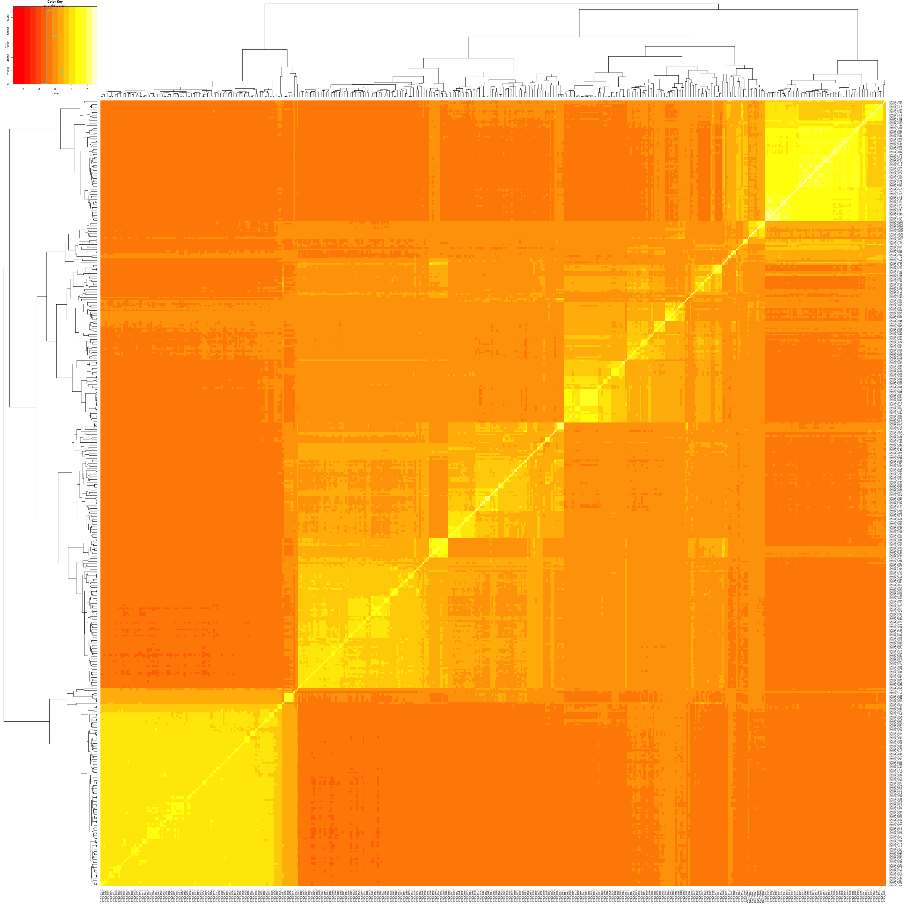
14.2 Duplicates
We can use the results from our kinship matrix to identify potential duplicates within our data. The existence of duplicates in a data set can mean different things. A sample may be genotyped multiple times or accidentally re-entried as a new individual sample and it is important to identify these errors. However, we can also find cases where the samples belong to different individuals but present no genetic variation, which can hint towards inbred lines or clonal lines. Moreover, duplicates inflate sample sizes, which can give us false confidence on GWAS or other statistical analyses. We will use the kinshipDuplicates() function from our package, which returns a list object with our kinship matrix, a data frame with our potential duplicates, and plots of the distribution of diagonal and off-diagonal values from our kinship matrix.
kinshipDuplicates(geno, threshold, method = "vanRaden", save = FALSE, kinship = NULL)
geno: our genotype matrixthreshold: a similarity threshold to differentiate our duplicatesmethod: set to"vanRaden"by default, accepts"astle","IBS", and"identity"save: defaults to FALSE, if TRUE, saves as a text filekinship: defaults to NULL, if we have already produced a kinship matrix we can define this parameter with it
# Identifying duplicates by setting a similarity threshold and using the ICARDA package
duplicates <- kinshipDuplicates(matrix, threshold = 0.99, kinship = kinshipMat)

# Printing potential duplicates along with their kinship and correlation
head(duplicates$potentialDuplicates)
Indiv.A Indiv.B Value Corr
1 ICARDA_G1416 ICARDA_G0226 1.623916 0.9988232
2 ICARDA_G0052 ICARDA_G0043 1.784647 0.9984566
3 ICARDA_G0140 ICARDA_G0059 1.840917 0.9983279
4 ICARDA_G0110 ICARDA_G0098 1.808388 0.9982951
5 ICARDA_G0119 ICARDA_G0098 1.807323 0.9980452
6 ICARDA_G0291 ICARDA_G0217 1.622423 0.9979949# Printing histograms with the distribution of diagonal and off-diagonal values
duplicates$plots[[1]]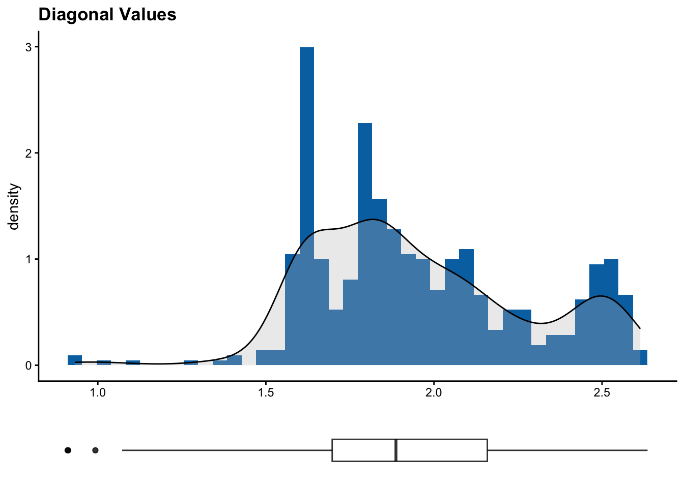
[[2]]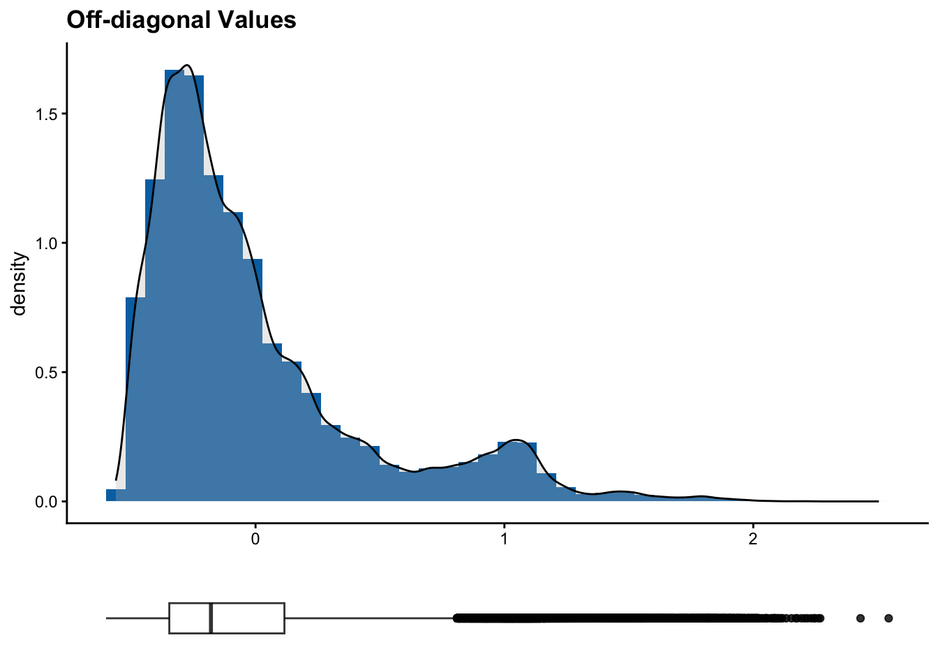
The diagonal of a kinship matrix is the self-relatedness of each individual. Most kinship estimators normalize values such that they are close to 1 or 0.5 according to scaling. Deviations may represent uneven SNP quality, duplicates or inbreeding. Off-diagonal entries are pairwise kinship estimates between two different individuals. These values are often closer to 0 , meaning the individuals are unrelated. Positive values mean the individuals share more alleles than expected by chance, and negative values mean the individuals are less related than expected. Clusters in a heatmap or in off-diagonal values often represent subpopulations.
If we decide we want to filter our data according to the potential duplicates we identified, we can use the kinshipFilter() function from the ICARDA package. This function requires our genotype matrix, our data frame with potential duplicates, and our kinship matrix. This will give us a filtered version of our SNP matrix and kinship matrix. We can also choose to save the matrix locally as a text file by setting the save parameter as TRUE, which is set to FALSE by default.
filteredMatrix <- kinshipFilter(matrix, duplicates$potentialDuplicates, kinshipMat)