# Importing filtered genotypic data
matrix <- read.table("data/FilteredBarley.txt", sep = "\t", header = TRUE,
                     row.names = 1, check.names = FALSE)
# SNP matrix has to have individuals in rows and markers as columns
# for the posterior functions
matrix <- t(matrix)

# Importing metadata
metadata <- read_excel("data/BarleyMetadata.xlsx")

# Defining our subgroups
popSet <- as.factor(metadata$countryOfOriginCode[metadata$Individual
%in% rownames(matrix)])17 Module 4.4: Phylogenetic Trees
Besides exploring population structure, we may want to explore evolutionary relationships between individuals. We can use phylogenetic trees to infer common ancestry, track lineage divergence, and reconstruct evolutionary and adaptation history. We will focus on distance-based methods. These require us to construct a genetic distance matrix, from which a tree is constructed by clustering similar individuals.
17.1 Tree Methods
Neighbor Joining (NJ): builds an unrooted tree by minimizing the total branch length. It is fast and scaleable, often used for SNP data.
Unweighted Pair Group Method with Arithmetic Mean (UPGMA): builds a rooted, ultrametric tree, meaning all leaves are at an equal distance from the root. It clusters taxa based on average pairwise distances and assumes a constant rate of evolution.
17.2 Distance types
Nei’s distance [
nei.dist()]: Measures genetic divergence based on allele frequencies. Very common in population genetics.Euclidean distance [
bitwise.dist()]: Based on geometric distance in multidimensional space.Reynolds’ distance [
reynolds.dist()]: Reynolds’ distance measures genetic differentiation due to drift and it as the main evolutionary force. Good for closely related populations.Rogers’ distance [
rogers.dist()]: Scaled version of the standard Euclidean distance applied to allele frequency data.Edwards’ distance [
edwards.dist()]: Measures the cosine of the angle between allele frequency vectors.Prevosti’s distance [
provesti.dist()]: Based on the absolute difference in allele frequencies between two populations.
17.3 Creating our tree
We will be using the phyloTree() function from our package to create our phylogenetic tree. This function uses framework from the poppr package to construct the phylogenetic tree.
phyloTree(geno, treeType, distanceType, samples, path): returns a phylo type object
geno: our genotype matrixtreeType: a text or function that can calculate a tree from a distance matrix, defaults to “upgma”distanceType: a character or function defining the distance to be applied, defaults tonei.dist()samples: a number of bootstrap replicates, defaults to 100path: file path to save tree in Newick format
The output tree can be plotted using the plot() function. We can define the type of visualization in the type parameter, which defaults to "phylogram" and accepts "cladogram", "fan", "unrooted", "radial" or "tidy". The produced Newick file can be visualized better with tools such as iTOL, which allows for more visualization and annotation options.
# Creating NJ tree from Nei's distance (1 sample for time purposes)
tree <- phyloTree(matrix, treeType = "nj", distanceType = nei.dist, samples = 1,
                  path = here("output", "tree.txt"))
Warning in aboot(alleleFreq, tree = treeType, distance = distanceType, sample =
samples, : Some branch lengths of the tree are negative. Normalizing branches
according to Kuhner and Felsenstein (1994)
Calculating bootstrap values... done.# Creating vector of colors for better visualization
popColors <- rainbow(nlevels(popSet))[as.numeric(popSet)]
# Plotting tree
plot(tree, main = "NJ Tree with Bootstrap", type = "phylogram", tip.color = popColors, cex = 0.1)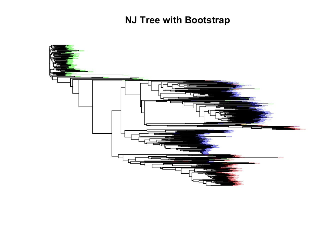
# Creating NJ tree from Nei's distance (1 sample for time purposes)
tree <- phyloTree(matrix, treeType = "upgma", distanceType = nei.dist, samples = 1,
path = "output/tree.txt")
# Creating vector of colors for better visualization
popColors <- rainbow(nlevels(popSet))[as.numeric(popSet)]

# Plotting tree
plot(tree, main = "NJ Tree with Bootstrap", type = "phylogram", tip.color = popColors, cex = 0.1)