9 Module 2.1: Loading Data - ICARDA Barley Example

9.1 Introduction to the Dataset

In this module, we’ll learn how to load typical phenotypic data into R. We’ll use a real-world example: data from a study on 275 barley accessions conducted at ICARDA in 2019. This dataset contains various measurements related to agronomic traits, grain quality, and morphological characteristics.

Why this dataset? It’s representative of the kind of multi-trait data breeders work with. It allows us to practice loading, inspecting, and performing basic summaries on realistic data. This data comes from ICARDA’s valuable work in crop improvement for dry areas.

Column Descriptions (Partial List - full list would be in a data dictionary): * Taxa: The identifier for each barley accession (genotype). * Area: Grain area (e.g., mm²). * B_glucan: Beta-glucan content (%), a quality trait. * DTH: Days to Heading (days), an agronomic trait. * Fe: Iron content in grain (ppm), a nutritional trait. * FLA: Flag Leaf Area (cm²). * GY: Grain Yield (e.g., t/ha or kg/plot - units should always be known!). * PH: Plant Height (cm). * Protein: Grain protein content (%). * TKW: Thousand Kernel Weight (grams). * Zn: Zinc content in grain (ppm). * (And many others related to grain morphology and plant characteristics…)

Our goal is to load this data (which is typically stored in a file like a CSV or Excel sheet) into an R data frame so we can start analyzing it.

9.2 Setting Up: Libraries and File Path

First, we need to load the R packages that help us read data. Even though we have previously installed and loaded all packages we will need, in case you are only focusing on reading data, the readr package (part of tidyverse) is excellent for reading text files like CSVs.

Remember our RStudio Project setup! We will assume the data file is saved in the data/ subfolder of our project.

# Load the necessary libraries
# 'tidyverse' includes 'readr' (for read_csv) and 'dplyr' (for glimpse, etc.)
library(tidyverse)

── Attaching core tidyverse packages ──────────────────────── tidyverse 2.0.0 ──
✔ dplyr     1.1.4     ✔ readr     2.1.5
✔ forcats   1.0.0     ✔ stringr   1.5.2
✔ ggplot2   4.0.0     ✔ tibble    3.3.0
✔ lubridate 1.9.4     ✔ tidyr     1.3.1
✔ purrr     1.1.0     
── Conflicts ────────────────────────────────────────── tidyverse_conflicts() ──
✖ dplyr::filter() masks stats::filter()
✖ dplyr::lag()    masks stats::lag()
ℹ Use the conflicted package (<http://conflicted.r-lib.org/>) to force all conflicts to become errors

9.3 Reading the CSV File

Let’s say our barley data is stored in a CSV file named icarda_barley_2019_pheno.csv.

# Define the path to our data file (relative to the project root)
barley_data_file_path <- "data/icarda_barley_2019_pheno.csv"

# Use read_csv() from the readr package to load the data
barley_pheno_data <- read_csv(barley_data_file_path)

9.4 First Look: Inspecting the Loaded Data

It’s CRUCIAL to always inspect your data immediately after loading it to make sure it looks correct.

head(): Shows the first few rows (default is 6).
dim(): Shows the dimensions (number of rows, number of columns).
glimpse() (from dplyr): A great way to see column names, their data types, and the first few values. Better than str() for tibbles.
summary(): Provides basic summary statistics for each column (Min, Max, Mean, Median, Quartiles for numeric; counts for character/factor).

9.5 Understanding Data Types in Our Barley Data

When glimpse() runs, you’ll see types like: * Taxa: Should be <chr> (character) as it’s an identifier. * Area, B_glucan, DTH, GY, PH, etc.: Should mostly be <dbl> (double-precision numeric) as they are measurements.

If read_csv misinterprets a numeric column as character (e.g., if there’s a text entry like “missing” in a numeric column), you’ll need to clean that data or specify column types during import using the col_types argument in read_csv().

glimpse(barley_pheno_data)

Rows: 275
Columns: 24
$ Taxa        <chr> "G1", "G2", "G3", "G4", "G5", "G7", "G8", "G9", "G12", "G1…
$ Area        <dbl> 22.72177, 23.07877, 19.93612, 23.32083, 19.54859, 22.96829…
$ B_glucan    <dbl> 6.848584, 7.430943, 4.012621, 6.091926, 7.307811, 7.267738…
$ Circularity <dbl> 1.887915, 1.780070, 1.555492, 2.300471, 1.896487, 1.752493…
$ Diameter    <dbl> 5.366522, 5.403555, 5.034355, 5.420909, 4.981714, 5.422541…
$ DTH         <dbl> 75.89584, 70.17532, 74.19461, 74.39462, 77.66037, 72.65420…
$ Fe          <dbl> 29.67685, 31.59088, 34.15825, 31.44544, 30.31127, 30.61605…
$ FLA         <dbl> 16.586760, 7.966124, 7.592350, 18.753322, 16.532845, 18.40…
$ FLH         <dbl> 82.77116, 62.36145, 61.81653, 69.77661, 64.38496, 78.08801…
$ GpS         <dbl> 44.70886, 25.25222, 25.72167, 66.23116, 54.63221, 26.63211…
$ GWS         <dbl> 1.6156277, 1.0563208, 0.9516462, 2.5202010, 1.2044795, 1.0…
$ GY          <dbl> 1.3747605, 1.3735596, 0.9054266, 0.7614383, 0.8827177, 2.0…
$ HW          <dbl> 57.65487, 64.41055, 69.41048, 55.35590, 53.65940, 64.98411…
$ Length      <dbl> 10.542981, 10.106793, 8.565790, 11.920853, 9.781558, 9.968…
$ Length_Wid  <dbl> 3.313525, 3.013035, 2.524445, 3.833381, 3.305421, 2.978634…
$ PdH         <dbl> 91.09761, 63.65600, 68.75482, 69.50663, 64.10002, 80.59519…
$ PdL         <dbl> 8.1320940, 1.0341930, 6.5555050, 0.9639243, -0.6416490, 2.…
$ Perimeter   <dbl> 29.07010, 28.33654, 24.57919, 32.21194, 27.02846, 28.03643…
$ PH          <dbl> 96.76140, 70.56720, 77.16486, 79.22446, 71.78375, 88.70248…
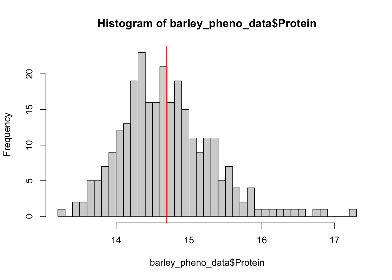
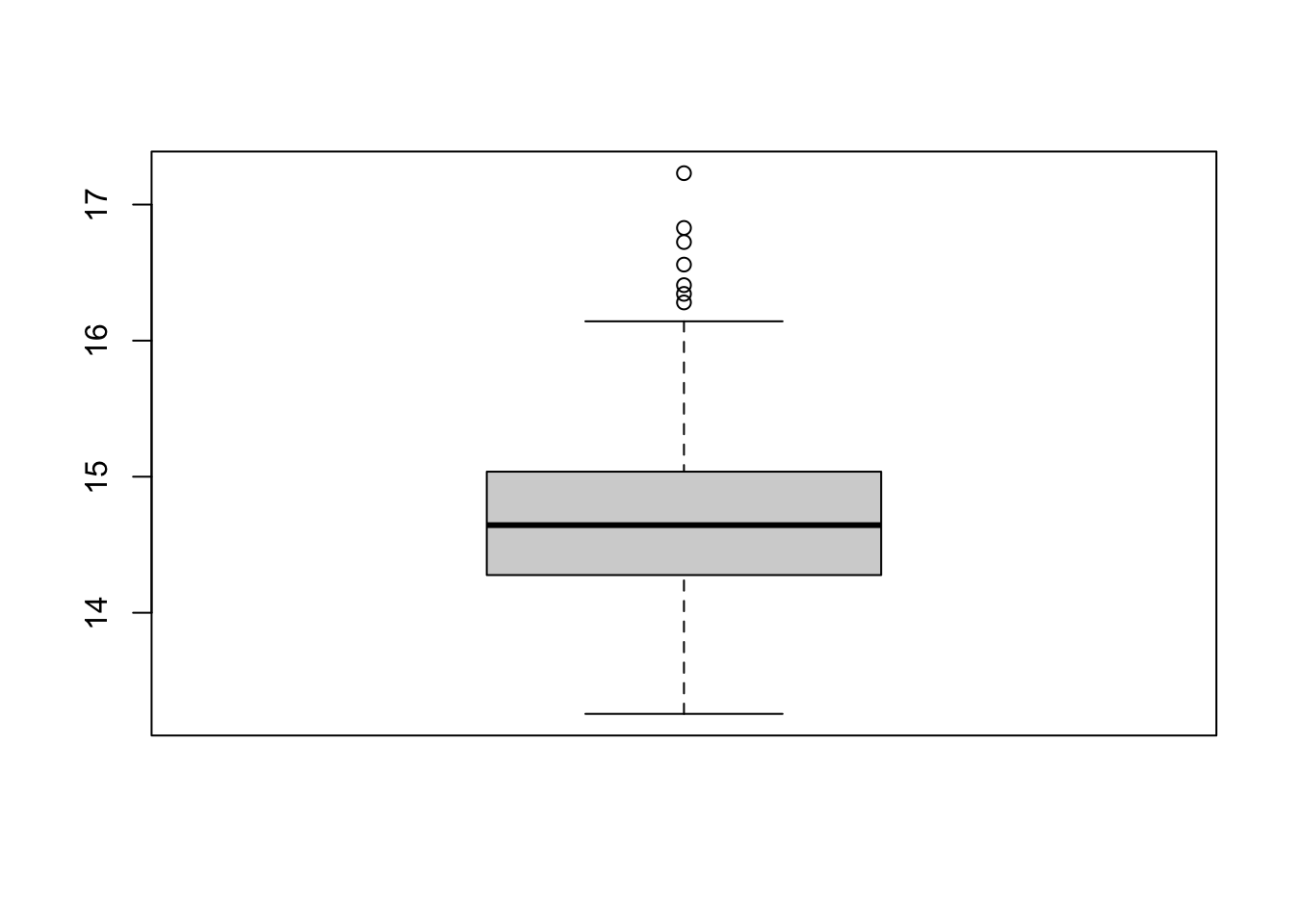
$ Protein     <dbl> 14.06372, 14.16090, 15.23294, 14.34877, 14.46224, 14.31356…
$ SL          <dbl> 5.343668, 6.804813, 8.074976, 10.039594, 7.526454, 8.31457…
$ TKW         <dbl> 28.48964, 35.00164, 31.95561, 27.27054, 24.64983, 33.83401…
$ width       <dbl> 3.251696, 3.439623, 3.455571, 3.204069, 3.000305, 3.429043…
$ Zn          <dbl> 31.21179, 34.21217, 25.50724, 32.24918, 33.58773, 33.92710…

9.6 Quick Summary of a Specific Trait

Let’s say we are interested in Grain Yield (GY).

# Access the GY column
yield_values <- barley_pheno_data$GY

# Calculate some basic statistics
# na.rm=TRUE ignores missing values in calculation
mean_yield <- mean(yield_values, na.rm = TRUE)
min_yield <- min(yield_values, na.rm = TRUE)
max_yield <- max(yield_values, na.rm = TRUE)
sd_yield <- sd(yield_values, na.rm = TRUE)

# Print statistics
print(paste("Average Grain Yield (GY):", round(mean_yield, 2)))

[1] "Average Grain Yield (GY): 1.19"

print(paste("Minimum Grain Yield (GY):", round(min_yield, 2)))

[1] "Minimum Grain Yield (GY): 0.5"

print(paste("Maximum Grain Yield (GY):", round(max_yield, 2)))

[1] "Maximum Grain Yield (GY): 2.47"

print(paste("Standard Deviation of GY:", round(sd_yield, 2)))

[1] "Standard Deviation of GY: 0.31"

# How many accessions do we have yield data for (non-missing)?
num_yield_obs <- sum(!is.na(yield_values))
print(paste("Number of accessions with GY data:", num_yield_obs))

[1] "Number of accessions with GY data: 275"

9.7 Visualizing data

We can visualize the distribution of a specific variable using histograms and box plots.

# Plotting histogram
hist(barley_pheno_data$Protein, breaks = 50)
# Adding mean
abline(v = mean(barley_pheno_data$Protein), col = "red")
# Adding median
abline(v = median(barley_pheno_data$Protein), col = "blue")

# Plotting box plot
boxplot(barley_pheno_data$Protein)

We can evaluate if there is any general structure that can be identified through PCA.

# Scale and run PCA (without our 1st ID column)
pca_res <- prcomp(barley_pheno_data[,-1], scale. = TRUE)

# Summary: variance explained
summary(pca_res)

Importance of components:
                          PC1    PC2    PC3    PC4     PC5     PC6     PC7
Standard deviation     2.6325 2.1211 1.6450 1.4170 1.24105 1.05346 0.90836
Proportion of Variance 0.3013 0.1956 0.1177 0.0873 0.06696 0.04825 0.03587
Cumulative Proportion  0.3013 0.4969 0.6146 0.7018 0.76882 0.81707 0.85294
                           PC8     PC9    PC10    PC11    PC12    PC13    PC14
Standard deviation     0.85950 0.78036 0.71730 0.69099 0.60831 0.50649 0.46036
Proportion of Variance 0.03212 0.02648 0.02237 0.02076 0.01609 0.01115 0.00921
Cumulative Proportion  0.88506 0.91154 0.93391 0.95467 0.97076 0.98191 0.99112
                          PC15    PC16    PC17    PC18    PC19    PC20    PC21
Standard deviation     0.26978 0.21679 0.19348 0.15733 0.11306 0.06560 0.05557
Proportion of Variance 0.00316 0.00204 0.00163 0.00108 0.00056 0.00019 0.00013
Cumulative Proportion  0.99429 0.99633 0.99796 0.99904 0.99959 0.99978 0.99991
                          PC22    PC23
Standard deviation     0.04048 0.01871
Proportion of Variance 0.00007 0.00002
Cumulative Proportion  0.99998 1.00000

# PCA scores (samples)
scores <- as.data.frame(pca_res$x)

# PCA loadings (traits contribution)
loadings <- as.data.frame(pca_res$rotation)

# Plot first two PCs
plot(scores$PC1, scores$PC2,
     xlab = paste0("PC1 (", round(summary(pca_res)$importance[2,1]*100, 1), "%)"),
     ylab = paste0("PC2 (", round(summary(pca_res)$importance[2,2]*100, 1), "%)"),
     main = "PCA Scatterplot")