# Importing filtered genotypic data
matrix <- read.table("data/FilteredBarley.txt", sep = "\t", header = TRUE,
                     row.names = 1, check.names = FALSE)

# SNP matrix has to have individuals in rows and markers as columns
# for the posterior functions
matrix <- t(matrix)

# Importing metadata
metadata <- read_excel("data/BarleyMetadata.xlsx")16 Module 4.3: Population Structure
Population structure in crop breeding refers to the presence of clusters or subpopulations that are genetically distinct from each other. The subpopulations may reflect geography, breeding history, natural selection, gene pools, or other differentiating factors. The subgroups are identified by differences in allele frequencies.
16.1 Why is it important?
Allows us to detect subpopulations and understand genetic diversity
Can be used to control bias in GWAS or other genomic prediction models (by including structure information as covariates), as not accounting for structure may lead to spurious associations (false-positives)
Acknowledging structure can help guide breeding programs
16.2 Common methods
STRUCTURE / ADMIXTURE: Uses Bayesian clustering or Maximum Likelihood (ML) estimation to assign individuals into subpopulations, including admixture proportions for each individual.
Principal Component Analysis (PCA): Used to reduce dimentionality of large data sets, and to visualize overall diversity and major genetic groupings.
Spatial Principal Component Analysis (sPCA): Incorporates spatial information (geographic location) into traditional PCA, meaning it seeks to maximize spatial autocorrelation along with variation. It allows us to identify global and local trends.
Discriminant Analysis of Principal Components (DAPC): Used to assign individuals to groups, provide a visual assessment of between-population differentiation and the contribution of individual alleles to the population structure.
Sparse Non-negative Matrix Factorization (sNMF): Fast algorithm used to infer structure by estimating ancestry coefficients. Allows us to evaluate levels of admixture. More efficient than STRUCTURE for large data sets.
All methods are complementary to each other and using them in combination can help us fully understand structure in our data.
| Want to explore structure quickly? | PCA |
| Want to analyze spatial genetic variation? | sPCA |
| Need to classify individuals into groups? | DAPC |
| Need to estimate admixture proportions? | sNMF |
We will be using functions from our package to carry out and visualize most of these analyses.
16.3 PCA
PCA reduces our large genotype matrix into principal components which capture the variation in our data. We will use the PCAFromMatrix() function from our package. This function uses the PCA framework from the ade4 package. This function returns a list with three objects, the first one being a PCA, the second one being a data frame with the variance explained by each component, and the third one being a plot of the PCA results (1st and 2nd PCs).
PCAFromMatrix(geno, subgroups = NULL): returns a pca object from genotype matrix
geno: our genotype matrixsubgroups: defaults to NULL, can be replaced with a vector of our factor information
# We will be guiding our analysis by the 'countryOfOriginCode' metadata column
# Defining our subgroups
popSet <- as.factor(metadata$countryOfOriginCode[metadata$Individual
                                                 %in% rownames(matrix)])
# Running our pca using our genotype data and groups
pca <- PCAFromMatrix(matrix, popSet)

# Printing pca object
pca$pca
Duality diagramm
class: pca dudi
$call: dudi.pca(df = x.genInd, center = FALSE, scale = FALSE, scannf = FALSE,
nf = round(ncol(geno)/3, 0))
$nf: 487 axis-components saved
$rank: 487
eigen values: 288 231.5 102.3 71 37.18 ...
vector length mode content
1 $cw 12141 numeric column weights
2 $lw 488 numeric row weights
3 $eig 487 numeric eigen values
data.frame nrow ncol content
1 $tab 488 12141 modified array
2 $li 488 487 row coordinates
3 $l1 488 487 row normed scores
4 $co 12141 487 column coordinates
5 $c1 12141 487 column normed scores
other elements: cent norm # Printing PC variation
head(pca$var) PC Variance CumulativeVar
1 1 17.004415 17.00442
2 2 13.666554 30.67097
3 3 6.040506 36.71148
4 4 4.191208 40.90268
5 5 2.195083 43.09777
6 6 1.665563 44.76333# Plotting pca results
pca$plot16.4 sPCA
We will be using the sPCA() function from our package. This function uses the sPCA framework from the adegenet package. It returns a list with our sPCA object, a plot of the obtained eigenvalues, results and plots for the global test and results and plots for the local test. The obtained sPCA result can be plotted using the sPCAMapPlot() function.
sPCA(geno, subgroups = NULL, xy, eigenPlot = TRUE, tests = TRUE): returns sPCA from genotype data
geno: our genotype matrixsubgroups: defaults to NULL, can be replaced with a vector of our factor informationxy: a two column longitude - latitude vector or data frameeigenPlot: defaults to TRUE, plots the resulting eigenvaluestests: defaults to TRUE, carries out global and local tests
sPCAMapPlot(spca, geno, xy, axis = 1, pos = TRUE): plots our sPCA results on a map
spca: our spca objectgeno: our genotype matrixxy: a two column longitude - latitude vector or data frameaxis: defaults to 1 (our first axis), we can choose any other axis to plotpos: defaults to TRUE to plot the positive values, can be set to FALSE to plot the negative values
# Running sPCA
spca <- sPCA(matrix, subgroups = popSet, xy = metadata[,c("LON","LAT")],
             eigenPlot = TRUE, tests = FALSE)

# Plotting our obtained eigenvalues
spca$eigenPlot

# Plotting global test results
spca$globalTest

# Plotting local test results
spca$localTest

# Plotting our results in a map
sPCAMapPlot(spca$spca, matrix, xy = metadata[,c("LON","LAT")],
            axis = 1, pos = TRUE)
The global test tests whether the genetic structure detected is globally significant, while the local test tests identifies which individuals or sites contribute significantly (hotspots).
16.5 DAPC
DAPC requires the user to define a range of subpopulation numbers for which to perform the analyses. To do this, we can calculate different k-statistics to guide our choice of this range. We will be using our kMeansStats() function, which allows us to choose between "BIC", "AIC" or "WCC" for our desired k-statistic. This function outputs a data frame with our k-statistic values, and a plot. We will then use our DAPC() function on our genotype data, which uses the DAPC framework from the adegenet package. This function outputs a list with the dapc object and a data frame with the explained variances. An additional plot can also be produced.
kMeansStats(geno, pca = NULL, maxK, stat): returns test statistic results for different K values
geno: our genotype matrixpca: defaults to NULL, can be replaced by a pca object to skip over creating a new PCAmaxK: the maximum number of K subpopulations for which to calculate k-statisticsstat: type of k-statistic to calculate
DAPC(geno, krange, subgroups = NULL, pca = NULL, dapcPlot = FALSE): performs DAPC
geno: our genotype matrixkrange: a range of K valuessubgroups: defaults to NULL, can be replaced with a vector of our factor informationpca: defaults to NULL, can be replaced by a pca object to skip over creating a new PCAdapcPlot: defaults to FALSE, if TRUE, an output plot is produced
# Calculating our K statistics
BICDAPC <- kMeansStats(matrix, pca$pca, 10, "BIC")

# Plotting K statistic
BICDAPC$statPlot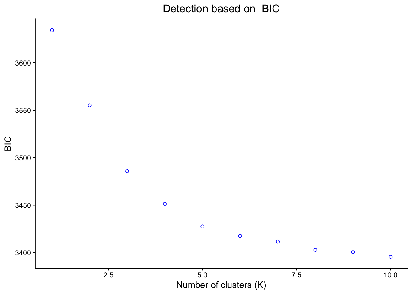
# Running DAPC
DAPC <- DAPC(matrix, krange = 3:7, pca = pca$pca, subgroups = popSet,
             dapcPlot = TRUE)

# Plotting DAPC results
DAPC$dapcPlot
Our resulting DAPC outputs group assignments for each individual, which can be visualized through a composition plot.
DAPCCompoPlot(DAPC, geno, krange, subgroups = NULL): returns a composition plot of DAPC results
DAPC: a dapc objectgeno: our genotype matrixkrange: a range of K valuessubgroups: defaults to NULL, can be replaced with a vector of our factor information
DAPCCompoPlot(DAPC$dapc, matrix, krange = 3:7, subgroups = popSet)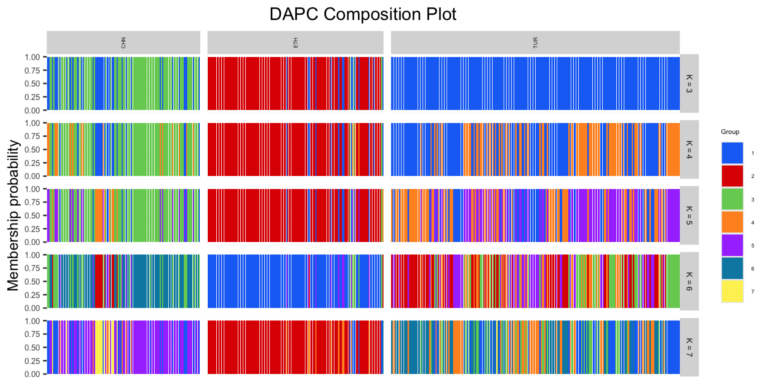
We can also produce a frequency plot from our DAPC. This helps us understand the relationship between the produced group assignments and prior group information we may have.
DAPCFreqPlot(DAPC, subgroups): produces a frequency plot of our DAPC results
DAPC: a single dapc objectsubgroups: a vector of our factor information
# For k = 3, which is our first object in our DAPC object
DAPCFreqPlot(DAPC$dapc[[1]], subgroups = popSet)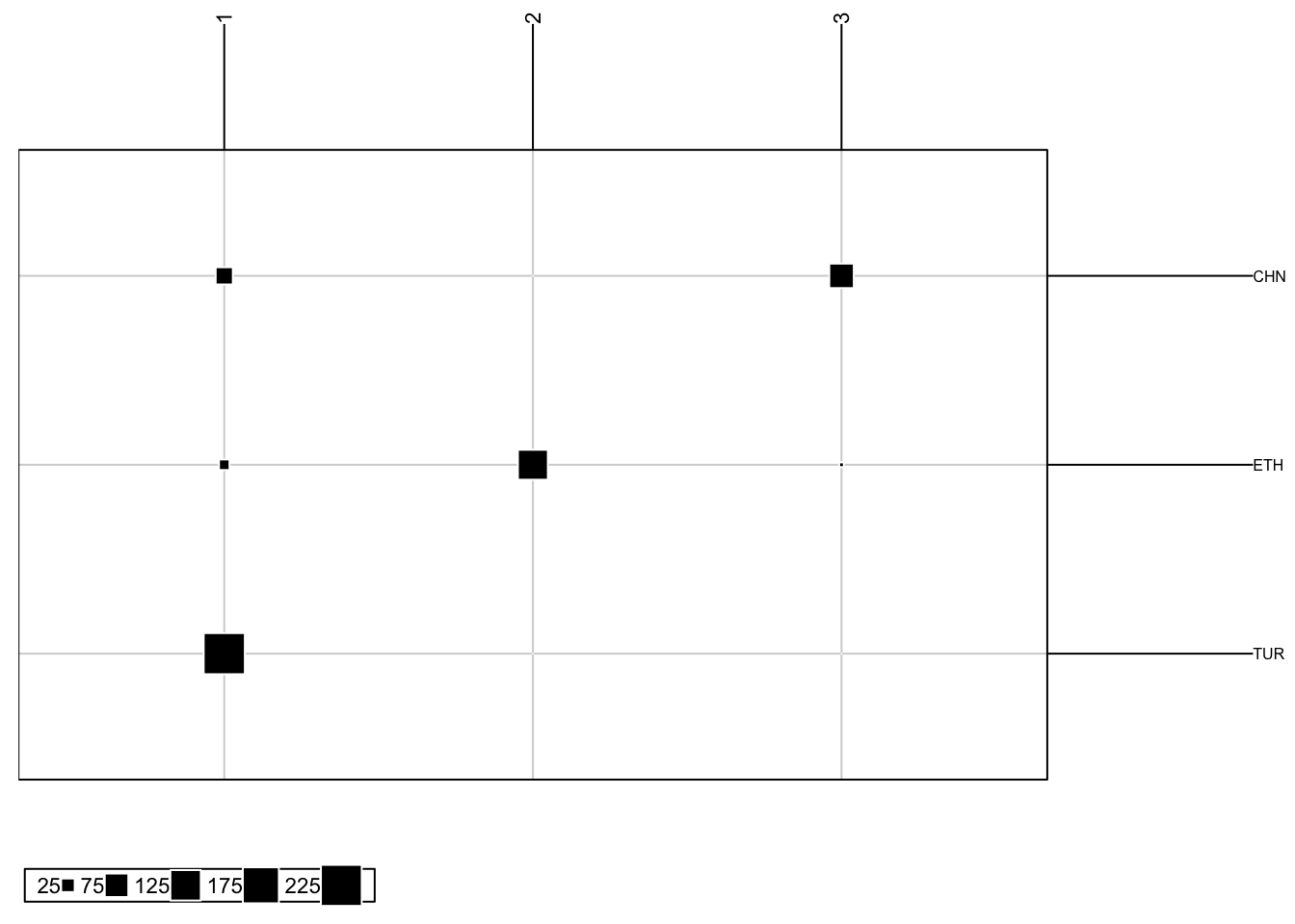
16.6 sNMF
sNMF is used to estimate admixture proportions: how much of an individual’s genome comes from different ancestral populations. This means that individuals are not just assigned to a population, instead membership probabilities (admixture coefficients) are calculated. We will be using functions from our package to carry out these analyses. The framework they use comes from the LEA package. Prior to estimating ancestry coefficients, this package requires us to create a geno type object, which we will create using the write.geno.mod() function. We can then run our main function using sNMFFunction(), which outputs a list with our snmf object, a matrix with the produced ancestry coefficients, and a data frame with cross-entropy values. The latter can guide our choice of best K value.
write.geno.mod(geno, output.file): creates geno type object from genotype matrix
geno: our genotype matrixoutput.file: file path where to save our object
sNMFFunction(geno, file, maxK, subgroups = NULL, cePlot = TRUE): outputs ancestry coefficients
geno: our genotype matrixfile: file path of geno objectmaxK: the maximum number of K subpopulationssubgroups: defaults to NULL, can be replaced with a vector of our factor informationcePlot: defaults to TRUE, outputs a plot of cross-entropy values
# Creating 'geno' object needed to run sNMF
write.geno.mod(matrix, "output/sNMFgenoBarley.geno")

# Running sNMF
sNMF <- sNMFFunction(matrix, subgroups = popSet, "output/sNMFgenoBarley.geno", maxK = 6, cePlot = TRUE)
We can visualize our membership probability results using a composition plot.
sNMFCompoPlot(sNMFmatrix, geno, krange, subgroups = NULL): returns a composition plot of admixture results
sNMFmatrix: ancestry coefficient matrixgeno: our genotype matrixkrange: a range of K valuessubgroups: defaults to NULL, can be replaced with a vector of our factor information
# Plotting composition plot
sNMFCompoPlot(sNMF$qmatrix, matrix, krange = 2:6, subgroups = popSet)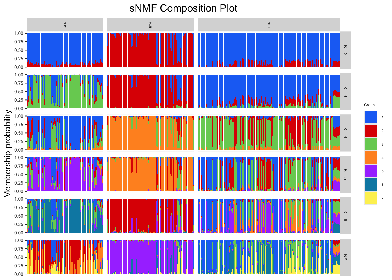
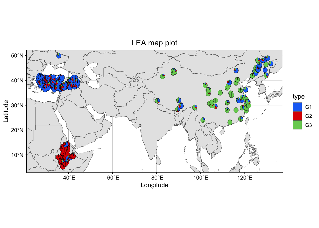
Finally, we can also visualize our sNMF results on a map by incorporating spatial information if available.
sNMFMapPlot(geno, sNMFObjectVar, xy, k, Xlim = NULL, Ylim = NULL): produces a map plot from ancestry coefficient results for a specific number of subgroups
geno: our genotype matrixsNMFObjectVar: a snmf objectxy: a two column longitude - latitude vector or data framek: a number K of subpopulationsXlim: defaults to NULL, can be replaced by a range of longitudes to zoom in the mapYlim: defaults to NULL, can be replaced by a range of latitudes to zoom in the map
# Plotting results in map
sNMFMapPlot(matrix, sNMF$snmf, xy = metadata[,c("LON","LAT")], 3)
Warning: Using `size` aesthetic for lines was deprecated in ggplot2 3.4.0.
ℹ Please use `linewidth` instead.
ℹ The deprecated feature was likely used in the scatterpie package.
Please report the issue to the authors.